What Is Interpolation?
Interpolation is a method used to determine values of particular elements that have a linear or some sort of relationship. For our purposes, the relationship is always linear.
Linear Interpolation Fundamental
With linear interpolation, you have "linear", which means that the interpolation is that of a line or a set of data that behaves like a line. In algebra, you have the line equation Y = MX + B and from this equation, you can generate a list of data points (X1, Y1), (X2, Y2), etc. that fit this equation.
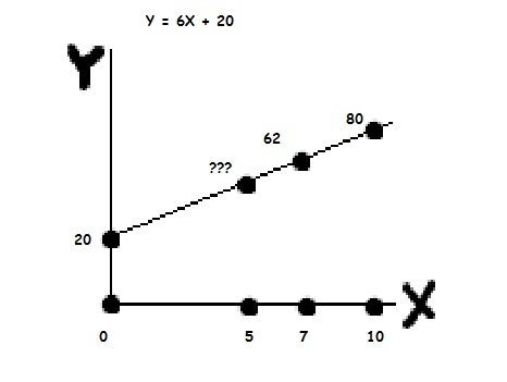 For example, you can have the equation Y = 6X + 20 and from this equation, you can get (0, 20), (10, 80), and (7, 62) as points on this line. Of course, there are more points on this line than those three. For any value of X, you can get a value of Y. For instance, if you were given X=5, you could find Y = 50 by using the line equation.
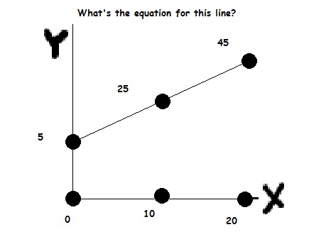
You can also reconstruct the line equation from a set of those points. If you had (0, 5), (10, 25), and (20, 45), then you can find the values for M and B. M would be the change in Y divided by the matching change in X, or rise over run as in Algebra. Either pair of points will give you the same value for M, which is 2. The value of B is found by taking any point and putting its X and Y back into the Y = MX + B, along with the newly found M. B = Y - MX, which will be 5. You could use this equation to find points as well. X = 5 yields Y = 15.
Linear Interpolation Basics
This is kind of what linear interpolation is, except we use a number X that ranges from 0 to 1 (making X to be like a percent). We will have at least two boundary values (the Y), and we use linear interpolation to get any value between those two points.
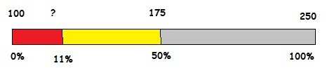 For example, with 100 and 250 as the two boundary values, a value of 0 for X means that Y = 100, and X = 1 means Y = 250. Intermediate values of X correspond to intermediate values of Y. X = 0.5 means Y = 175. But other values get progressively more difficult to eyeball, such as X = 0.11 (if you can get it, then linear interpolation is not hard at all).
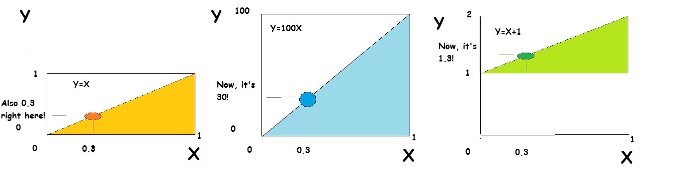
The easy case of interpolation is when the boundary values are 0 and 1, and the value of Y is simply the value of X (Y = X).
If we expand the maximum boundary condition upward so that our boundary is now 0 to H, then Y would be equal to H * X.
If we instead shifted the whole region upwards so that the boundary values are L to L + 1, Y would be X + L.
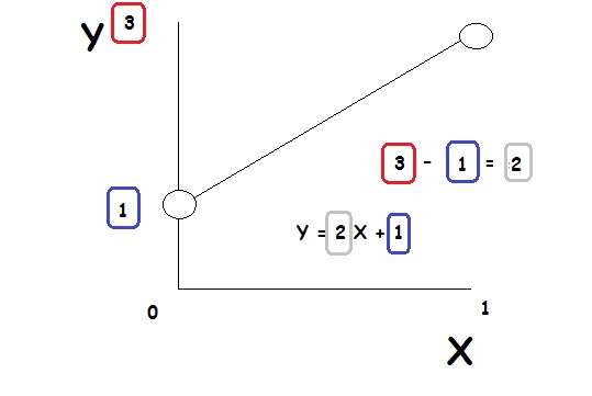 Now, how would these two combine? We'll set up a very simple case where the boundary is 1 to 3. This would mean that, as X increases from 0 to 1, Y increases from 1 to 3... therefore, since 3 - 1 = 2, Y is 2X plus some other value that doesn't depend on X. That would be one, since Y = 1 when X = 0.
Therefore Y = 2X + 1.
And in the general case, with boundaries of L to H, Y = (H - L)X + L.
This equation can also be manipulated to find what percent a given value of Y is along two boundary points, by simply solving for X instead of Y. This would give us the equation X = (Y - L) / (H - L), and I typically call this Reversed Linear Interpolation.
Double Linear Interpolation
Linear Interpolation by itself is quite useful, but using it twice is even more useful.
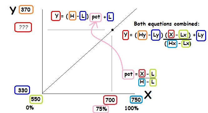 Consider that you have two pairs of boundary values (550 To 750 and 330 To 370, for example), and you want to figure out what 700 in the first range would correspond to in the second range. Now, 550 would correspond to 330 of course, and 750 would correspond to 370. What you would do is first use X = (Y - L) / (H - L) to find the percentage of the 700 in the first range (in this case .75, or 75%), then you apply the other formula: Y = (H - L)X + L to find what X corresponds to in the second range (360). Formulaically, these can be combined into one formula for finding what a certain value in one range would correspond to in the second range. If the first range's bounds are from Li to Hi, and the second range's bounds are from Lf to Hf, then the first reversed interpolation would be X = (Y - Li) / (Hi - Li) and, after substituting into the second expression, we end up with Y2 = [(Hf - Lf)(Y - Li) / (Hi - Li)] + Lf, which doesn't look as nice as the other two, but gets the job done. Remember that Li and Hi are the boundary values that correspond to the current value of Y. There's also the other version that interpolates from percent to percent, but it is less useful. X2 = ((H - L)X + L - A) / (Z - A)
Uses of Interpolation
Interpolation has lots of nice uses. Its handy at filling in missing gaps on some tables of data. From a programming standpoint, they work excellently with custom progressbars and scrollbars. Many times, a VB programmer wants to make a custom progressbar by drawing a rectangle, and this rectangle can go from some initial width L to a final width H (50 to 3600, for example), and it also has to correspond with some data, like a loop that loads N (let's say it loads 200) files. Therefore, when we are finished with Y files (Y is just any number of files), we can do our linear interpolation to represent what the width of the rectangle should be. Here, we'd do the double interpolation, with Li = 0, Hi = 200, Lf = 50, and Hf = 3600, and our formula would look like:
Y2 = [(3600 - 50)(Y - 0) / (200 - 0)] + 50, simplified to [3550Y / 200] + 50, or 17.75Y + 50. In VB, this would be
TheShape.Width = 17.75 * LV + 50 where LV is either the loop variable or the count of files loaded. The 17.75 can be altered to 18 for simplying the multiplication.
With scrollbars, you typically interpolate with the scrollbar value, scrollbar maximum, scrollbar minimum, and the two boundaries where you want the display to be located at the minimum and maximum of the scrollbar. The scrollbar maximum and minimum can be adjusted. Typically, I go for 0 To 100 as the scrollbar boundaries - these values correspond to Li and Hi. The display boundaries are arbitrary, just ask yourself two questions: "where should the display be when the scrollbar is at the top" (this is Lf), and "where should the display be when the scrollbar is at the bottom" (this is Hf). The scrolling practically takes care of itself. With Y as the scrollbar value, our interpolation is ready to be written. (Note: I am using Double Interpolation again)
Y2 = [(Hf - Lf)(Y - 0) / (100 - 0)] + Lf = [(Hf - Lf)Y / 100] + Lf, or in VB:
TheFrame.Top = (Hf - Lf) * Y / 100 + Lf. Again, Lf and Hf are arbitrary values that you decide on.
Return to the Line Equation (extra)
Remember that all of these operations are linear. Upon examination of Y2 = [(Hf - Lf)(Y - Li) / (Hi - Li)] + Lf, you find that it can be expanded into
Y2 = [(Hf - Lf)Y - (Hf - Lf)Li] / (Hi - Li) + Lf = [(Hf - Lf) / (Hi - Li)]Y - [(Hf - Lf)Li / (Hi - Li)] + Lf. This is just like Y = MX + B, except we have Y2 instead of Y and Y instead of X. M = [(Hf - Lf) / (Hi - Li)] and B = - [(Hf - Lf)Li / (Hi - Li)] + Lf = Lf - M*Li.